Leveraging Bayesian Optimization in Design of Experiments (DoE) for Enhanced Crystallization Process Development

Youcef Leghrib

02 Jul 2024 • 3 min read

Active learning starts with problem initialization, which includes defining the task and training a model on an initial set of labeled data. This is followed by sequential experimental selection, where the most informative data points are iteratively chosen from the unlabeled dataset using specific query strategies, thereby continuously improving the model's performance.

In the world of pharmaceutical manufacturing, optimizing the crystallization process is crucial for ensuring high-quality Active Pharmaceutical Ingredients (APIs). Traditional methods for optimizing experimental conditions can be time-consuming and resource-intensive. Enter Bayesian Optimization (BO) — a powerful machine learning technique that is transforming the Design of Experiments (DoE) by making the process more efficient and effective. In this blog, we will explore how BO can be applied in DoE, particularly for the crystallization processes in pharmaceutical development.

What is Bayesian Optimization?

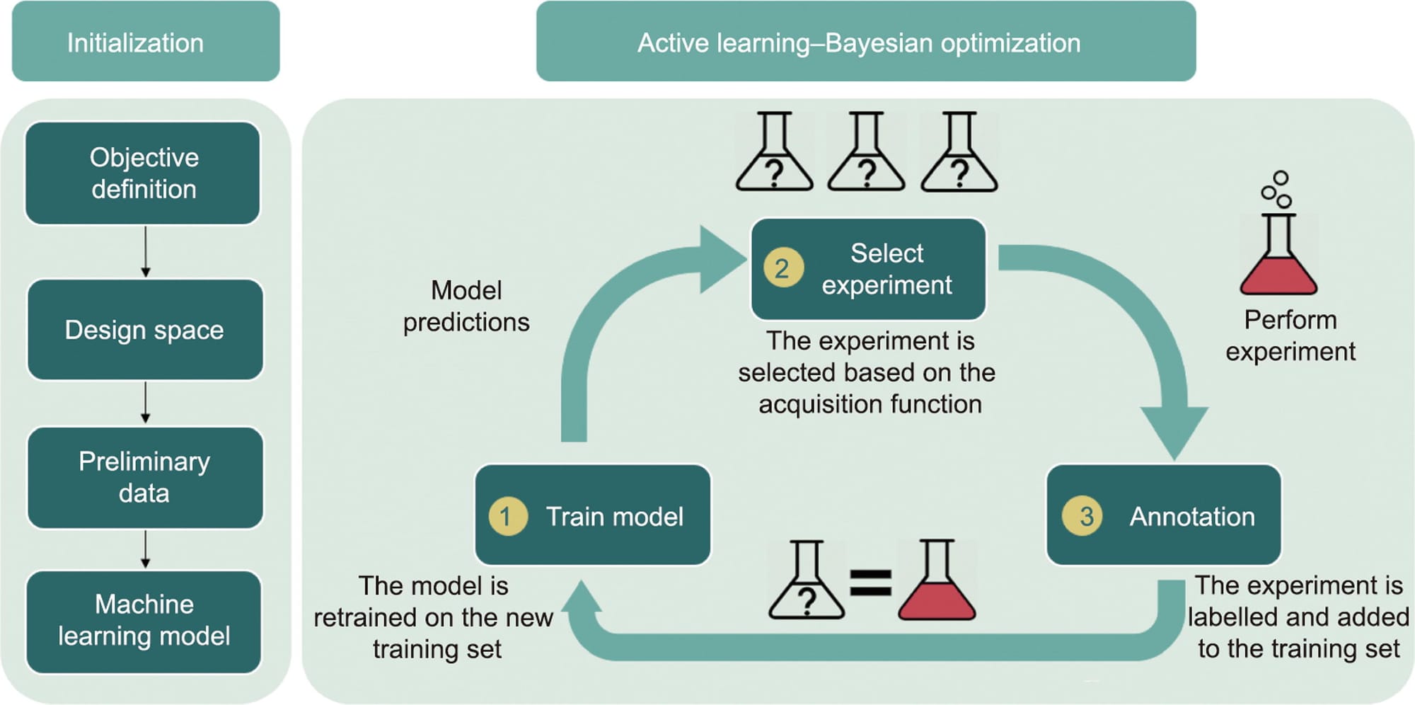
Bayesian Optimization is a strategy for finding the maximum or minimum of an objective function that is expensive to evaluate. It is particularly useful when dealing with black-box functions where the underlying mechanism is unknown. BO uses a surrogate model, typically a Gaussian Process, to model the objective function and an acquisition function to decide where to sample next.

Why Use Bayesian Optimization in DoE?

Traditional DoE methods often rely on factorial designs or response surface methodologies, which can become impractical as the number of variables increases. BO, on the other hand, excels in high-dimensional spaces and efficiently handles the trade-off between exploration and exploitation. This makes it an ideal choice for optimizing complex processes like crystallization.

Applying BO to Crystallization Processes

Step 1: Define the Objective Function

The objective function in a crystallization process could be to maximize yield, optimize crystal size distribution (CSD), or improve crystal morphology. For instance, if we aim to maximize yield, we define the yield as our objective function.

Step 2: Set Up the Experimental Domain

The domain defines the range of experimental conditions. In crystallization, this might include parameters like cooling rate, seed mass, and supersaturation.

Step 3: Choose the Surrogate Model

The surrogate model approximates the objective function. Gaussian Processes are commonly used due to their flexibility and ability to provide uncertainty estimates.

Step 4: Define the Acquisition Function

The acquisition function guides the selection of the next experimental point by balancing exploration (sampling new areas) and exploitation (refining known good areas). Common acquisition functions include Expected Improvement (EI) and Upper Confidence Bound (UCB).

Step 5: Run the Optimization

By iteratively updating the surrogate model and selecting new experimental points, BO efficiently converges to the optimal conditions.

Example Implementation

Here’s an example of how BO can be implemented using Python and the GPyOpt library:

import pandas as pd
from sklearn.ensemble import RandomForestRegressor
import GPyOpt
from GPyOpt.methods import BayesianOptimization

def load_data(file_path):
    df = pd.read_excel(file_path)
    return df

def main():
    file_path = '/Users/youcef/Desktop/DoE_Scaled_Samples_with_Yield.xlsx'

    df_samples = load_data(file_path)
    
    # Ensure there are no empty rows
    df_samples = df_samples.dropna(subset=["Cooling Rate (C°/min)", "Seed Mass (%)", "SS", "Yield"])

    # Separate the features (X) and target (y)
    X = df_samples[["Cooling Rate (C°/min)", "Seed Mass (%)", "SS"]]
    y_yield = df_samples["Yield"]

    # Train the Random Forest Regressor
    model_yield = RandomForestRegressor(n_estimators=100, random_state=42)
    model_yield.fit(X, y_yield)

    # Define the objective function for yield
    def objective_yield(x):
        # x is a 2D array with shape (n_samples, n_features)
        predictions = model_yield.predict(x)
        # Since we want to maximize the yield, return the negative value
        return -predictions

    # Define the domain (bounds) for the parameters
    domain = [
        {'name': 'Cooling Rate (C°/min)', 'type': 'continuous', 'domain': (0.1, 0.5)},
        {'name': 'Seed Mass (%)', 'type': 'continuous', 'domain': (1, 5)},
        {'name': 'SS', 'type': 'continuous', 'domain': (1.2, 1.5)}
    ]

    # Set up the Bayesian Optimization
    optimizer = BayesianOptimization(f=objective_yield, domain=domain, acquisition_type='EI')

    # Run the optimization to propose the next experiment
    optimizer.run_optimization(max_iter=10)

    # Print the suggested next experiment
    print("Suggested next experiment parameters:")
    print("Cooling Rate (C°/min):", optimizer.x_opt[0])
    print("Seed Mass (%):", optimizer.x_opt[1])
    print("SS:", optimizer.x_opt[2])

if __name__ == "__main__":
    main()

Benefits of Using BO in DoE

Efficiency: BO reduces the number of experiments needed by focusing on the most promising areas.
Flexibility: It can handle different types of objectives and constraints.
Adaptability: BO can easily be adapted to new objectives or experimental conditions as they arise.

Bayesian Optimization offers a robust and efficient approach to optimizing complex processes like crystallization in pharmaceutical development. By leveraging BO, researchers can significantly reduce the time and resources required for DoE, leading to faster and more reliable results. As machine learning continues to evolve, we can expect BO to play an increasingly important role in experimental optimization across various fields.

Call to Action

Interested in implementing Bayesian Optimization in your experimental designs? Get started with GPyOpt and see the difference it can make in your research and development processes. For more information and resources, check out the GPyOpt documentation.

References

- Rasmussen, C.E., & Williams, C.K.I. (2006). Gaussian Processes for Machine Learning. MIT Press.
- Frazier, P. I. (2018). A Tutorial on Bayesian Optimization. arXiv:1807.02811
- Ureel, Yannick et al. “Active Machine Learning for Chemical Engineers: A Bright Future Lies Ahead.” Engineering (Beijing, China) 27 (2023): 23–30.